Datan ryhmittely ja kuvailevat analyysit
Kertausta
Miksi R:ää?
Kolme syytä:
- lisensointi
- internet
- lisensointi
licence()##
## This software is distributed under the terms of the GNU General
## Public License, either Version 2, June 1991 or Version 3, June 2007.
## The terms of version 2 of the license are in a file called COPYING
## which you should have received with
## this software and which can be displayed by RShowDoc("COPYING").
## Version 3 of the license can be displayed by RShowDoc("GPL-3").
##
## Copies of both versions 2 and 3 of the license can be found
## at https://www.R-project.org/Licenses/.
##
## A small number of files (the API header files listed in
## R_DOC_DIR/COPYRIGHTS) are distributed under the
## LESSER GNU GENERAL PUBLIC LICENSE, version 2.1 or later.
## This can be displayed by RShowDoc("LGPL-2.1"),
## or obtained at the URI given.
## Version 3 of the license can be displayed by RShowDoc("LGPL-3").
##
## 'Share and Enjoy.'# This software is distributed under the terms of the GNU General
# Public License, either Version 2, June 1991 or Version 3, June 2007.
# The terms of version 2 of the license are in a file called COPYING
# which you should have received with
# this software and which can be displayed by RShowDoc("COPYING").
# Version 3 of the license can be displayed by RShowDoc("GPL-3").
#
# Copies of both versions 2 and 3 of the license can be found
# at https://www.R-project.org/Licenses/.
#
# A small number of files (the API header files listed in
# R_DOC_DIR/COPYRIGHTS) are distributed under the
# LESSER GNU GENERAL PUBLIC LICENSE, version 2.1 or later.
# This can be displayed by RShowDoc("LGPL-2.1"),
# or obtained at the URI given.
# Version 3 of the license can be displayed by RShowDoc("LGPL-3").
#
# 'Share and Enjoy.'Erityisesti Linux kernelistä tunnettu GNU General Public License (GPL) lienee ehkä kuuluisin vapaan lähdekoodin lisenssi. GPL on esimerkki copyleft (käyttäjänoikeus) lisenssistä. Copyleft-lisenssit ovat vapaan lähdekoodin lisenssejä jotka vaativat, että johdannaisteokset ovat myös copyleft-lisenssin alaisia. Copyleft-lisenssejä sanotaan tämän vuoksi myös tarttuviksi lisensseiksi. Kuten suomenkielinen nimi antaa ymmärtää, copyleftin tarkoitus on suojella loppukäyttäjää. Se tekee tämän kieltämällä uusien rajoitteiden lisäämisen lisenssiin ja näin kannustamalla kehittäjiä suosimaan vapaata lähdekoodia.
GPL sallii teoksen levityksen ja muokkauksen, kunhan seuraavia ehtoja noudatetaan:
- Lisenssiä ei saa muuttaa tai poistaa
- Muokkauksista pitää lisätä huomio
- Ohjelman tulee sisältää tieto lisenssistä
- Lähdekoodi pitää tehdä saataville kaikille, joille ohjelma on levitetty
- Johdannaisteokset tulee lisensoida samalla lisenssillä
GPL ei ole kuitenkaan EULA, eli se ei koske ohjelmiston käyttäjää. Ehdot koskevat ainoastaan levittäjiä. Omia muutoksia ei myöskään tarvitse julkaista kenelle tahansa, vaan ainoastaan niille kenelle muokatusta ohjelmasta on annettu kopio. Eli sisäiseen käyttöön tehtyjä muutoksia ei ole pakko julkaista.
Lähde: Sofokus: Avoin lähdekoodi – Tiedätkö mitä rajoituksia se asettaa ohjelmistosi käytölle?
Avoimen lisensoinnin seuraukset
- Contributed packages https://cran.r-project.org/web/packages/
- On the growth of CRAN packages http://blog.revolutionanalytics.com/2016/04/cran-package-growth.html
- The Popularity of Data Analysis Software http://r4stats.com/articles/popularity/
- The Impressive Growth of R : https://stackoverflow.blog/2017/10/10/impressive-growth-r/
- Microsoft R: MRAN https://mran.microsoft.com/open
- IBM Watson RStudio: https://dataplatform.cloud.ibm.com/docs/content/wsj/analyze-data/rstudio-overview.html
- Oracle R Distibution https://www.oracle.com/technetwork/database/database-technologies/r/r-distribution/overview/index.html
Datan manipuloinnin perusteet dplyr-paketilla
Kerrataan data-manipulaation perusverbit dplyr-paketista.
filter()- valitse rivejä datastaselect()- valitse muuttujiaarrange()- järjestä rivit uudelleenmutate()- luo uusia muuttujia olemassaolevista muuttujistagroup_by()- mahdollistaa yllä olevien viiden verbin käytön ryhmittäisen käytönsummarise()- tiivistä muuttujan arvo yhteen lukuun
Tidyverse-maailmassa yllä olevista kuudesta verbistä voidaan puhua datamanipulaation kielenä.
Kaikki toimivat samalla tapaa
- Ensimmäinen argumentti on data
- Seuraavat argumentit kuvaavat mitä datalle tehdään käyttäen muuttujanimiä ilman lainausmerkkejä
- Tulos on aina
tibble/data.frame
Eli käyttäen kotitehtävistä tuttua dataa..
library(tidyverse)
sw <-dplyr::starwars
sw
## # A tibble: 87 x 13
## name height mass hair_color skin_color eye_color birth_year gender
## <chr> <int> <dbl> <chr> <chr> <chr> <dbl> <chr>
## 1 Luke… 172 77 blond fair blue 19 male
## 2 C-3PO 167 75 <NA> gold yellow 112 <NA>
## 3 R2-D2 96 32 <NA> white, bl… red 33 <NA>
## 4 Dart… 202 136 none white yellow 41.9 male
## 5 Leia… 150 49 brown light brown 19 female
## 6 Owen… 178 120 brown, gr… light blue 52 male
## 7 Beru… 165 75 brown light blue 47 female
## 8 R5-D4 97 32 <NA> white, red red NA <NA>
## 9 Bigg… 183 84 black light brown 24 male
## 10 Obi-… 182 77 auburn, w… fair blue-gray 57 male
## # … with 77 more rows, and 5 more variables: homeworld <chr>,
## # species <chr>, films <list>, vehicles <list>, starships <list>…voidaan ensin valita ihmiset joilla on tukkaa
sw %>%
  dplyr::filter(species == "Human", hair_color != "none")
## # A tibble: 32 x 13
## name height mass hair_color skin_color eye_color birth_year gender
## <chr> <int> <dbl> <chr> <chr> <chr> <dbl> <chr>
## 1 Luke… 172 77 blond fair blue 19 male
## 2 Leia… 150 49 brown light brown 19 female
## 3 Owen… 178 120 brown, gr… light blue 52 male
## 4 Beru… 165 75 brown light blue 47 female
## 5 Bigg… 183 84 black light brown 24 male
## 6 Obi-… 182 77 auburn, w… fair blue-gray 57 male
## 7 Anak… 188 84 blond fair blue 41.9 male
## 8 Wilh… 180 NA auburn, g… fair blue 64 male
## 9 Han … 180 80 brown fair brown 29 male
## 10 Wedg… 170 77 brown fair hazel 21 male
## # … with 22 more rows, and 5 more variables: homeworld <chr>,
## # species <chr>, films <list>, vehicles <list>, starships <list>Sen jälkeen järjestetään data aineiston nousevaan järjestykseen syntymävuoden ja pituuden pituuden mukaan.
sw %>%
  dplyr::filter(species == "Human", hair_color != "none") %>%
  arrange(birth_year,height)
## # A tibble: 32 x 13
## name height mass hair_color skin_color eye_color birth_year gender
## <chr> <int> <dbl> <chr> <chr> <chr> <dbl> <chr>
## 1 Leia… 150 49 brown light brown 19 female
## 2 Luke… 172 77 blond fair blue 19 male
## 3 Wedg… 170 77 brown fair hazel 21 male
## 4 Bigg… 183 84 black light brown 24 male
## 5 Han … 180 80 brown fair brown 29 male
## 6 Land… 177 79 black dark brown 31 male
## 7 Boba… 183 78.2 black fair brown 31.5 male
## 8 Anak… 188 84 blond fair blue 41.9 male
## 9 Padm… 165 45 brown light brown 46 female
## 10 Beru… 165 75 brown light blue 47 female
## # … with 22 more rows, and 5 more variables: homeworld <chr>,
## # species <chr>, films <list>, vehicles <list>, starships <list>Sitten valitaan ainoastaan muuttujat name, height, mass, birth_year, gender, homeworld
sw %>%
  dplyr::filter(species == "Human", hair_color != "none") %>%
  arrange(birth_year,height) %>%
  select(name, height, mass, birth_year, gender, homeworld)
## # A tibble: 32 x 6
## name height mass birth_year gender homeworld
## <chr> <int> <dbl> <dbl> <chr> <chr>
## 1 Leia Organa 150 49 19 female Alderaan
## 2 Luke Skywalker 172 77 19 male Tatooine
## 3 Wedge Antilles 170 77 21 male Corellia
## 4 Biggs Darklighter 183 84 24 male Tatooine
## 5 Han Solo 180 80 29 male Corellia
## 6 Lando Calrissian 177 79 31 male Socorro
## 7 Boba Fett 183 78.2 31.5 male Kamino
## 8 Anakin Skywalker 188 84 41.9 male Tatooine
## 9 Padmé Amidala 165 45 46 female Naboo
## 10 Beru Whitesun lars 165 75 47 female Tatooine
## # … with 22 more rowsSen jölkeen luodaan uusi muuttuja painoindeksibmi joka siis paino jaettuna pituuden (metriä) neliöllä.
sw %>%
  dplyr::filter(species == "Human", hair_color != "none") %>%
  arrange(birth_year,height) %>%
  select(name, height, mass, birth_year, gender, homeworld) %>%
  dplyr::mutate(bmi = mass / (height/100)^2)
## # A tibble: 32 x 7
## name height mass birth_year gender homeworld bmi
## <chr> <int> <dbl> <dbl> <chr> <chr> <dbl>
## 1 Leia Organa 150 49 19 female Alderaan 21.8
## 2 Luke Skywalker 172 77 19 male Tatooine 26.0
## 3 Wedge Antilles 170 77 21 male Corellia 26.6
## 4 Biggs Darklighter 183 84 24 male Tatooine 25.1
## 5 Han Solo 180 80 29 male Corellia 24.7
## 6 Lando Calrissian 177 79 31 male Socorro 25.2
## 7 Boba Fett 183 78.2 31.5 male Kamino 23.4
## 8 Anakin Skywalker 188 84 41.9 male Tatooine 23.8
## 9 Padmé Amidala 165 45 46 female Naboo 16.5
## 10 Beru Whitesun lars 165 75 47 female Tatooine 27.5
## # … with 22 more rowsSitten lisätään uusi muuttuja jossa on homeworld-muuttujan luokittain painoindeksin keskiarvo (group_by yhdistettynä mutate:en luo uuden muuttujan joka riville)
sw %>%
  dplyr::filter(species == "Human", hair_color != "none") %>%
  arrange(birth_year,height) %>%
  select(name, height, mass, birth_year, gender, homeworld) %>%
  dplyr::mutate(bmi = mass / (height/100)^2) %>%
  group_by(homeworld) %>%
  mutate(mean_bmi = mean(bmi, na.rm = TRUE))
## # A tibble: 32 x 8
## # Groups: homeworld [14]
## name height mass birth_year gender homeworld bmi mean_bmi
## <chr> <int> <dbl> <dbl> <chr> <chr> <dbl> <dbl>
## 1 Leia Organa 150 49 19 female Alderaan 21.8 22.1
## 2 Luke Skywalker 172 77 19 male Tatooine 26.0 28.1
## 3 Wedge Antilles 170 77 21 male Corellia 26.6 25.7
## 4 Biggs Darklight… 183 84 24 male Tatooine 25.1 28.1
## 5 Han Solo 180 80 29 male Corellia 24.7 25.7
## 6 Lando Calrissian 177 79 31 male Socorro 25.2 25.2
## 7 Boba Fett 183 78.2 31.5 male Kamino 23.4 23.4
## 8 Anakin Skywalker 188 84 41.9 male Tatooine 23.8 28.1
## 9 Padmé Amidala 165 45 46 female Naboo 16.5 22.4
## 10 Beru Whitesun l… 165 75 47 female Tatooine 27.5 28.1
## # … with 22 more rowsJa aivan lopuksi vielä summataan alkuperäisestä datasta liittoon miesten ja naisten mediaanipainoindeksit. (group_by yhdistettynä summarise:en luo ryhmittäisen yhteenvedon ryhmittelevän muuttujan luokittain)
sw %>%
  dplyr::filter(species == "Human", hair_color != "none") %>%
  arrange(birth_year,height) %>%
  select(name, height, mass, birth_year, gender, homeworld) %>%
  dplyr::mutate(bmi = mass / (height/100)^2) %>%
  group_by(gender) %>%
  summarise(median_bmi = median(bmi, na.rm = TRUE))
## # A tibble: 2 x 2
## gender median_bmi
## <chr> <dbl>
## 1 female 21.8
## 2 male 24.8Ryhmittäiset yhteenvedot
aggregate(x = sw$height, by = list(sw$gender), mean, na.rm = TRUE)## Group.1 x
## 1 female 165.4706
## 2 hermaphrodite 175.0000
## 3 male 179.2373
## 4 none 200.0000sw %>%
dplyr::group_by(gender) %>%
dplyr::summarise(pituus_ka = mean(height, na.rm = TRUE),
eri_supujen_maara = n()) # dplyr## # A tibble: 5 x 3
## gender pituus_ka eri_supujen_maara
## <chr> <dbl> <int>
## 1 <NA> 120 3
## 2 female 165. 19
## 3 hermaphrodite 175 1
## 4 male 179. 62
## 5 none 200 2Tidy-datan perusteet
Lähde: http://r4ds.had.co.nz/tidy-data.html
“Happy families are all alike; every unhappy family is unhappy in its own way.” –– Leo Tolstoy
“Tidy datasets are all alike, but every messy dataset is messy in its own way.” –– Hadley Wickham
Alla sama data neljällä eri tavalla järjestettynä. Kaikissa datoissa on neljä muuttujaa country,year,population ja cases, mutta jokainen on järjestetty eri tavalla.
library(tidyverse)
data("table1")
table1
## # A tibble: 6 x 4
## country year cases population
## <chr> <int> <int> <int>
## 1 Afghanistan 1999 745 19987071
## 2 Afghanistan 2000 2666 20595360
## 3 Brazil 1999 37737 172006362
## 4 Brazil 2000 80488 174504898
## 5 China 1999 212258 1272915272
## 6 China 2000 213766 1280428583data("table2")
table2## # A tibble: 12 x 4
## country year type count
## <chr> <int> <chr> <int>
## 1 Afghanistan 1999 cases 745
## 2 Afghanistan 1999 population 19987071
## 3 Afghanistan 2000 cases 2666
## 4 Afghanistan 2000 population 20595360
## 5 Brazil 1999 cases 37737
## 6 Brazil 1999 population 172006362
## 7 Brazil 2000 cases 80488
## 8 Brazil 2000 population 174504898
## 9 China 1999 cases 212258
## 10 China 1999 population 1272915272
## 11 China 2000 cases 213766
## 12 China 2000 population 1280428583data("table3")
table3## # A tibble: 6 x 3
## country year rate
## * <chr> <int> <chr>
## 1 Afghanistan 1999 745/19987071
## 2 Afghanistan 2000 2666/20595360
## 3 Brazil 1999 37737/172006362
## 4 Brazil 2000 80488/174504898
## 5 China 1999 212258/1272915272
## 6 China 2000 213766/1280428583Kahdessa eri datassa:
data("table4a")
table4a
## # A tibble: 3 x 3
## country `1999` `2000`
## * <chr> <int> <int>
## 1 Afghanistan 745 2666
## 2 Brazil 37737 80488
## 3 China 212258 213766data("table4b")
table4b## # A tibble: 3 x 3
## country `1999` `2000`
## * <chr> <int> <int>
## 1 Afghanistan 19987071 20595360
## 2 Brazil 172006362 174504898
## 3 China 1272915272 1280428583Kaikki datat esittävät siis samaa pohjalla olevaa dataa, mutta ne eivät ole yhtä helppoja käyttää. Tidy data -ajattelussa pyritään yhdenmukaiseen datan rakenteeseen, tidy data:aan, jolloin datan kanssa työskentelyn helpottuu etenkin ns. tidyverse:en kuuluvilla työkaluilla joita tällä kurssillä käytämme. (Lue myös The tidy tools manifesto)
tidy-datan kolme ehtoa
Data on tidy kun se täyttää seuraavat toisistaan riippuvaiset kolme ehtoa:
- Jokainen muuttuja on omassa sarakkeessaan
- Jokainen havainto on omalla rivillään
- jokainen arvo on omassa solussaan
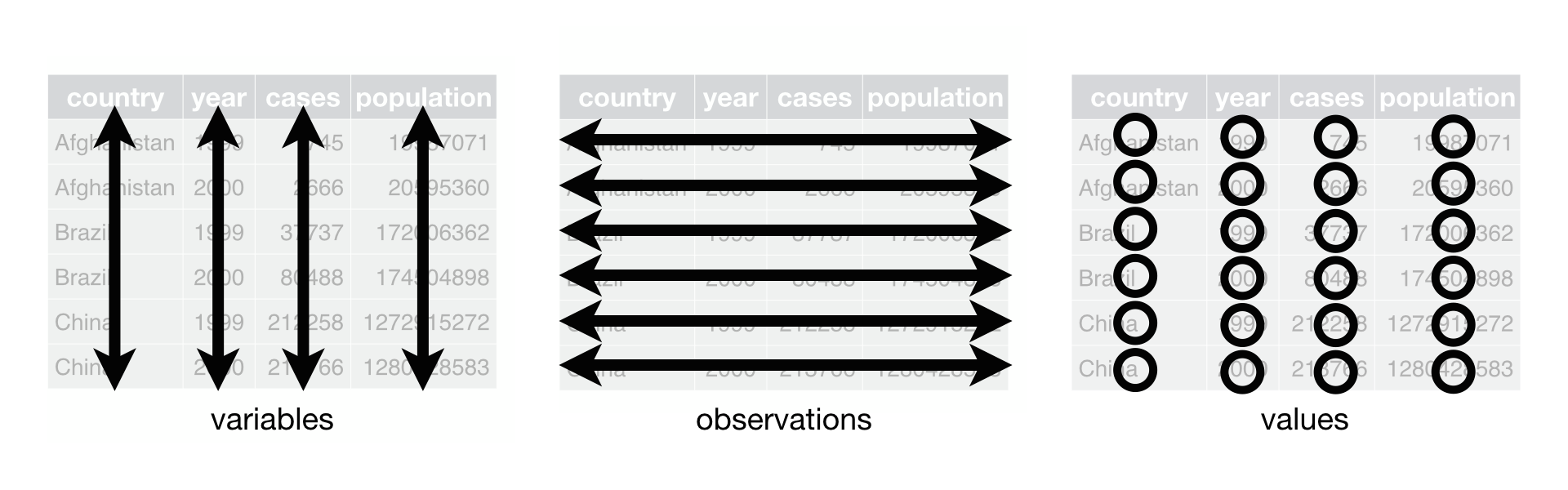
Kuva: Ehdot visualisoituna. Lähde: http://r4ds.had.co.nz/images/tidy-1.png
Koska ehdot ovat riippuvaisia toisistaan ja on mahdotonta täyttää kahta ilman kolmatta voi tidy:n datan ehtoina pitää seuraavia kahta:
- Jokainen data omana
tibble:nä (taidata.frame:na) - Jokainen muuttuja omassa sarakkeessaan
Yllä olevissa taulukoissa ainoastaan table1 on tidy ja siis ainoa, jossa kukin muuttuja on omassa sarakkeessaan.
Tidy:n datan hyödyt
- On ylipäätään hyödyllistä valita yksi johdonmukainen tapa datan säilyttämiseen. Kun datat ovat tidy-muodossa on helpompaa opetella ko. rakennetta edellyttäviä data-analyysin työkaluja.
- Muuttujien laittamisella omiin sarakkeihin pystyy myös hyödyntää paremmin R:n vektoroitua toimintatapaa.
Seuraavassa pari esimerkkiä siitä, miten helppoa on työskennellä tidy:n datan kanssa
table1 %>%
  mutate(vaestosuhde = cases / population * 10000)
## # A tibble: 6 x 5
## country year cases population vaestosuhde
## <chr> <int> <int> <int> <dbl>
## 1 Afghanistan 1999 745 19987071 0.373
## 2 Afghanistan 2000 2666 20595360 1.29
## 3 Brazil 1999 37737 172006362 2.19
## 4 Brazil 2000 80488 174504898 4.61
## 5 China 1999 212258 1272915272 1.67
## 6 China 2000 213766 1280428583 1.67table1 %>%
count(year, wt = cases)## # A tibble: 2 x 2
## year n
## <int> <int>
## 1 1999 250740
## 2 2000 296920library(ggplot2)
ggplot(table1, aes(x=year, y=cases)) +
geom_line(aes(group = country,colour = country)) +
geom_point(aes(colour = country))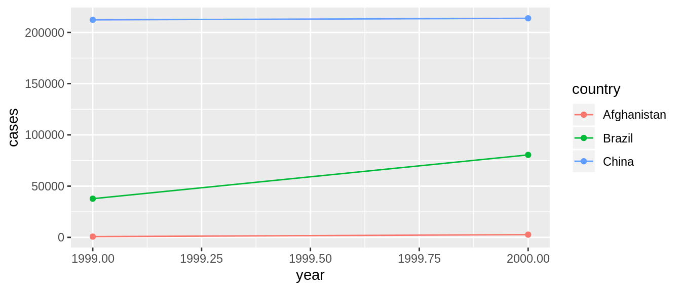
Lasketaan vastaava vaestosuhde ensin table2:sta
table2## # A tibble: 12 x 4
## country year type count
## <chr> <int> <chr> <int>
## 1 Afghanistan 1999 cases 745
## 2 Afghanistan 1999 population 19987071
## 3 Afghanistan 2000 cases 2666
## 4 Afghanistan 2000 population 20595360
## 5 Brazil 1999 cases 37737
## 6 Brazil 1999 population 172006362
## 7 Brazil 2000 cases 80488
## 8 Brazil 2000 population 174504898
## 9 China 1999 cases 212258
## 10 China 1999 population 1272915272
## 11 China 2000 cases 213766
## 12 China 2000 population 1280428583table2 %>%
tidyr::spread(., key = type, value = count, 3) %>%
dplyr::mutate(vaestosuhde = cases / population * 10000)## # A tibble: 6 x 5
## country year cases population vaestosuhde
## <chr> <int> <dbl> <dbl> <dbl>
## 1 Afghanistan 1999 745 19987071 0.373
## 2 Afghanistan 2000 2666 20595360 1.29
## 3 Brazil 1999 37737 172006362 2.19
## 4 Brazil 2000 80488 174504898 4.61
## 5 China 1999 212258 1272915272 1.67
## 6 China 2000 213766 1280428583 1.67ja sitten table4a:sta ja table4b:stä.
table4a## # A tibble: 3 x 3
## country `1999` `2000`
## * <chr> <int> <int>
## 1 Afghanistan 745 2666
## 2 Brazil 37737 80488
## 3 China 212258 213766table4b## # A tibble: 3 x 3
## country `1999` `2000`
## * <chr> <int> <int>
## 1 Afghanistan 19987071 20595360
## 2 Brazil 172006362 174504898
## 3 China 1272915272 1280428583t4a <- table4a %>% tidyr::gather(., key = year, value = cases, 2:3)
t4b <- table4b %>% tidyr::gather(., key = year, value = population, 2:3)
t4a %>% left_join(t4b) %>%
dplyr::mutate(vaestosuhde = cases / population * 10000)## # A tibble: 6 x 5
## country year cases population vaestosuhde
## <chr> <chr> <int> <int> <dbl>
## 1 Afghanistan 1999 745 19987071 0.373
## 2 Brazil 1999 37737 172006362 2.19
## 3 China 1999 212258 1272915272 1.67
## 4 Afghanistan 2000 2666 20595360 1.29
## 5 Brazil 2000 80488 174504898 4.61
## 6 China 2000 213766 1280428583 1.67Tidyr-paketin perusfunktiot
Luodaan esin data nimeltä tapaukset
tapaukset <- tibble::tibble(country = c("FR", "DE", "US", "FR", "DE", "US", "FR", "DE", "US"),
                 year = c(2011,2011,2011,2012,2012,2012,2013,2013,2013),
                 n = c(7000,5800,15000,6900,6000,14000,7000,6200,13000)) %>%
  spread(., year, n)
tapaukset
## # A tibble: 3 x 4
## country `2011` `2012` `2013`
## <chr> <dbl> <dbl> <dbl>
## 1 DE 5800 6000 6200
## 2 FR 7000 6900 7000
## 3 US 15000 14000 13000gather()
Leveässä muodossa olevan datan kokoaminen pitkään muotoon
tapaukset <- gather(data = tapaukset,  # data
                 key = year, # avainmuuttujan arp
                 value = n, # name of valut var
                 2:4) # variables NOT tidy
tapaukset
## # A tibble: 9 x 3
## country year n
## <chr> <chr> <dbl>
## 1 DE 2011 5800
## 2 FR 2011 7000
## 3 US 2011 15000
## 4 DE 2012 6000
## 5 FR 2012 6900
## 6 US 2012 14000
## 7 DE 2013 6200
## 8 FR 2013 7000
## 9 US 2013 13000`spread()
pitkän datan levittäminen
spread(data=tapaukset,  # data
       key=year, # class-var
       value=n) # amount
## # A tibble: 3 x 4
## country `2011` `2012` `2013`
## <chr> <dbl> <dbl> <dbl>
## 1 DE 5800 6000 6200
## 2 FR 7000 6900 7000
## 3 US 15000 14000 13000separate()
Luodaan data
myrskyt <- tibble::tibble(myrsky = c("Alberto", "Alex", "Allison", "Ana", "Arlene", "Arthur"),
                     tuulennopeus = c(110,45,65,40,50,45),
                     ilmanpaine = c(1007,1009,1005,1013,1010,1010),
                     pvm = as.Date(c("2000-08-03", "1998-07-27", "1995-06-03", "1997-06-30", "1999-06-11", "1996-06-17")))
myrskyt
## # A tibble: 6 x 4
## myrsky tuulennopeus ilmanpaine pvm
## <chr> <dbl> <dbl> <date>
## 1 Alberto 110 1007 2000-08-03
## 2 Alex 45 1009 1998-07-27
## 3 Allison 65 1005 1995-06-03
## 4 Ana 40 1013 1997-06-30
## 5 Arlene 50 1010 1999-06-11
## 6 Arthur 45 1010 1996-06-17myrskyt2 <- separate(data = myrskyt, col = pvm, into = c("vuosi", "kk", "pv"), sep = "-")
myrskyt2## # A tibble: 6 x 6
## myrsky tuulennopeus ilmanpaine vuosi kk pv
## <chr> <dbl> <dbl> <chr> <chr> <chr>
## 1 Alberto 110 1007 2000 08 03
## 2 Alex 45 1009 1998 07 27
## 3 Allison 65 1005 1995 06 03
## 4 Ana 40 1013 1997 06 30
## 5 Arlene 50 1010 1999 06 11
## 6 Arthur 45 1010 1996 06 17unite()
unite(myrskyt2, "paivamaara", vuosi, kk, pv, sep = "/")## # A tibble: 6 x 4
## myrsky tuulennopeus ilmanpaine paivamaara
## <chr> <dbl> <dbl> <chr>
## 1 Alberto 110 1007 2000/08/03
## 2 Alex 45 1009 1998/07/27
## 3 Allison 65 1005 1995/06/03
## 4 Ana 40 1013 1997/06/30
## 5 Arlene 50 1010 1999/06/11
## 6 Arthur 45 1010 1996/06/17list-columns ja nest()/unnest()
dplyr::starwars %>%
  select(name, films)
## # A tibble: 87 x 2
## name films
## <chr> <list>
## 1 Luke Skywalker <chr [5]>
## 2 C-3PO <chr [6]>
## 3 R2-D2 <chr [7]>
## 4 Darth Vader <chr [4]>
## 5 Leia Organa <chr [5]>
## 6 Owen Lars <chr [3]>
## 7 Beru Whitesun lars <chr [3]>
## 8 R5-D4 <chr [1]>
## 9 Biggs Darklighter <chr [1]>
## 10 Obi-Wan Kenobi <chr [6]>
## # … with 77 more rowsdplyr::starwars %>%
select(name, films) %>%
unnest() -> temp1
temp1## # A tibble: 173 x 2
## name films
## <chr> <chr>
## 1 Luke Skywalker Revenge of the Sith
## 2 Luke Skywalker Return of the Jedi
## 3 Luke Skywalker The Empire Strikes Back
## 4 Luke Skywalker A New Hope
## 5 Luke Skywalker The Force Awakens
## 6 C-3PO Attack of the Clones
## 7 C-3PO The Phantom Menace
## 8 C-3PO Revenge of the Sith
## 9 C-3PO Return of the Jedi
## 10 C-3PO The Empire Strikes Back
## # … with 163 more rowstemp1 %>%
group_by(name) %>%
nest(.key = films)## # A tibble: 87 x 2
## name films
## <chr> <list>
## 1 Luke Skywalker <tibble [5 × 1]>
## 2 C-3PO <tibble [6 × 1]>
## 3 R2-D2 <tibble [7 × 1]>
## 4 Darth Vader <tibble [4 × 1]>
## 5 Leia Organa <tibble [5 × 1]>
## 6 Owen Lars <tibble [3 × 1]>
## 7 Beru Whitesun lars <tibble [3 × 1]>
## 8 R5-D4 <tibble [1 × 1]>
## 9 Biggs Darklighter <tibble [1 × 1]>
## 10 Obi-Wan Kenobi <tibble [6 × 1]>
## # … with 77 more rowsTilastografiikkaa ggplot2-paketilla
Teoria
ggplot2-paketti perustuu Leland Wilkinsonin ajatukseen tilastografiikan kieliopista , josta kuvataaan teoksessa: Wilkinson, Leland, ja Graham Wills. 2005. The grammar of graphics. Springer.
Grammar of graphics (gg) -ajattelun ydin on että mikä tahansa tilastografiikka voidaan tehdä samoilla peruselementeillä:
- data
- geometrioita (
geoms) eli datapisteitä merkitseviä visuaalisia elementtejä - koordinaattijärjestelmä
Kuva rakennetaan kerros kerrokselta ja lopputuote voidaan tallentaa bittimappi tai vektorimuodoissa. (png vs. svg)
Dokumentaation top3:
Käytäntö
# Pohjakerros, jonka määritykset periytyvät muille kerroksille
p <- ggplot(data = sw,                  # Perusdatan määrittely
            mapping = aes(x = height,   # ja kuvattavien
                          y = mass,     # muuttujien mäppäys
                          color = gender)) + # (<aesthetics> = <var>)

# Geom-kerros eli käytettävä grafiikkatyyppi
  geom_point() +                        # Hajontakuvio

# Koordinaatit ja skaalat
  coord_cartesian() +                   # Suorakulmainen
  scale_y_log10() +                     # Logaritmimuunnos y-akselille

# Labelit ja guidet
  labs(title = "Esimerkkikuvio",        # Kuvion ja
       x = "pituus", y = "paino") +     # akselien otsikot
# Teemat
  theme_minimal() +                     # Valmis teema
  theme(legend.position = "bottom")     # Selitteen sijainti
# Kuvan tallentaminen
ggsave(filename = "./kuva.png", plot = p,
       height = 5, width = 6, dpi = 120)
p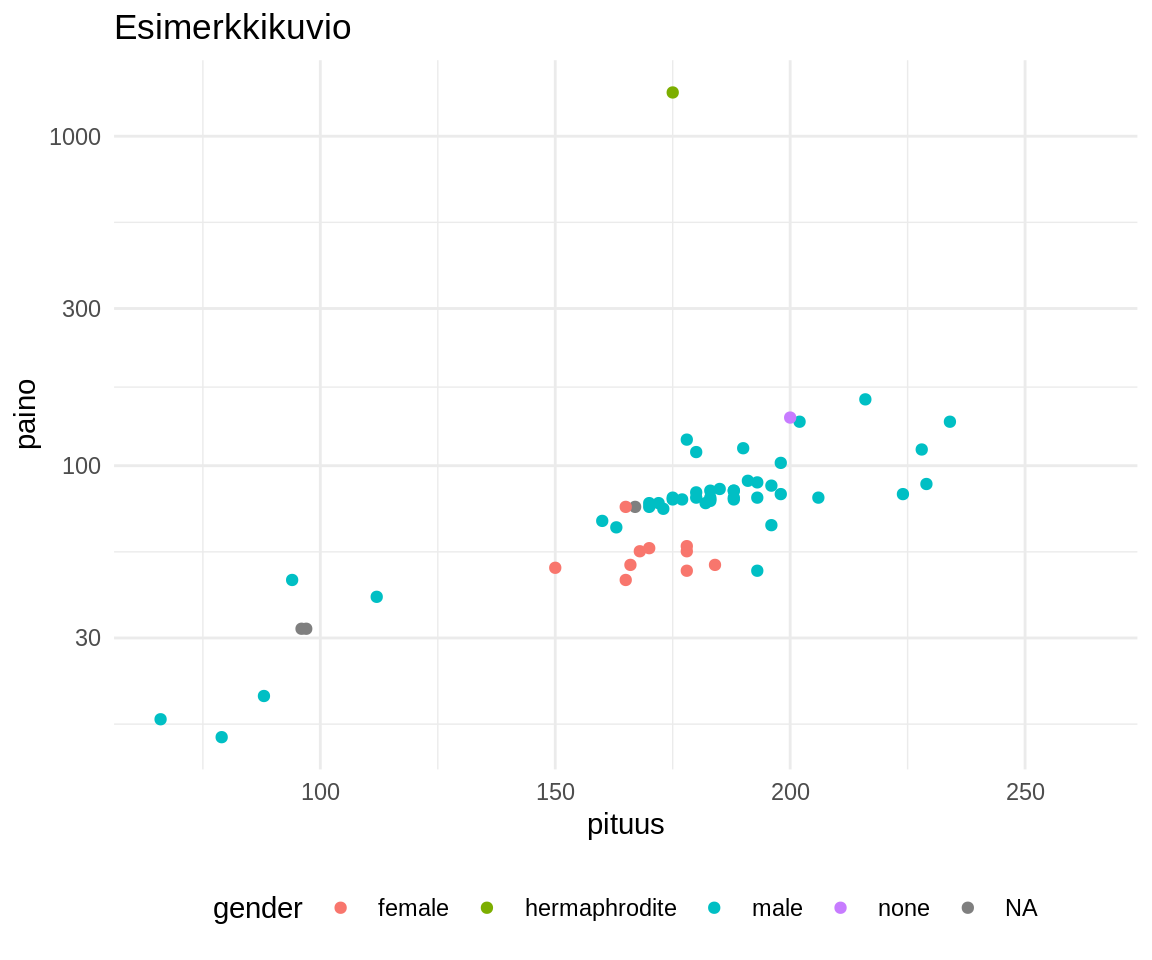
sw <- dplyr::starwars %>%
  mutate(species2 = ifelse(species == "Human", "ihminen", "elukka")) %>%
  # filteroidaan Jabba veks
  filter(name != "Jabba Desilijic Tiure") %>%
  # valitaan muuttujat
  select(name,height,mass,gender,species2)
head(sw)
## # A tibble: 6 x 5
## name height mass gender species2
## <chr> <int> <dbl> <chr> <chr>
## 1 Luke Skywalker 172 77 male ihminen
## 2 C-3PO 167 75 <NA> elukka
## 3 R2-D2 96 32 <NA> elukka
## 4 Darth Vader 202 136 male ihminen
## 5 Leia Organa 150 49 female ihminen
## 6 Owen Lars 178 120 male ihminenData tidy-muodossa, eli kukin muuttuja omassa sarakkeessaan ja kukin tapaus omalla rivillään!
Paketit
library(jsonlite) # json-muotoisen datan lukemiseen
library(readr) # .csv-datan lukemiseen
library(dplyr) # datan käsittelyyn
library(ggplot2) # grafiikkaan
Kuvion pohjadatan määrittäminen
ggplot(data = sw) #<<
Kuvattavien (mapping) muuttujien valinta mapping = aes()-funktio
ggplot(data = sw,
       mapping = aes(x = height, #<<
                     y = mass))  #<<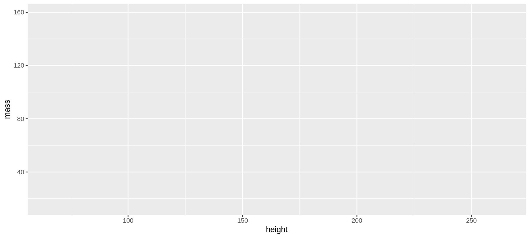
Geometrian lisääminen geom_point()
ggplot(data = sw,
       mapping = aes(x = height,
                     y = mass)) +
  geom_point() #<<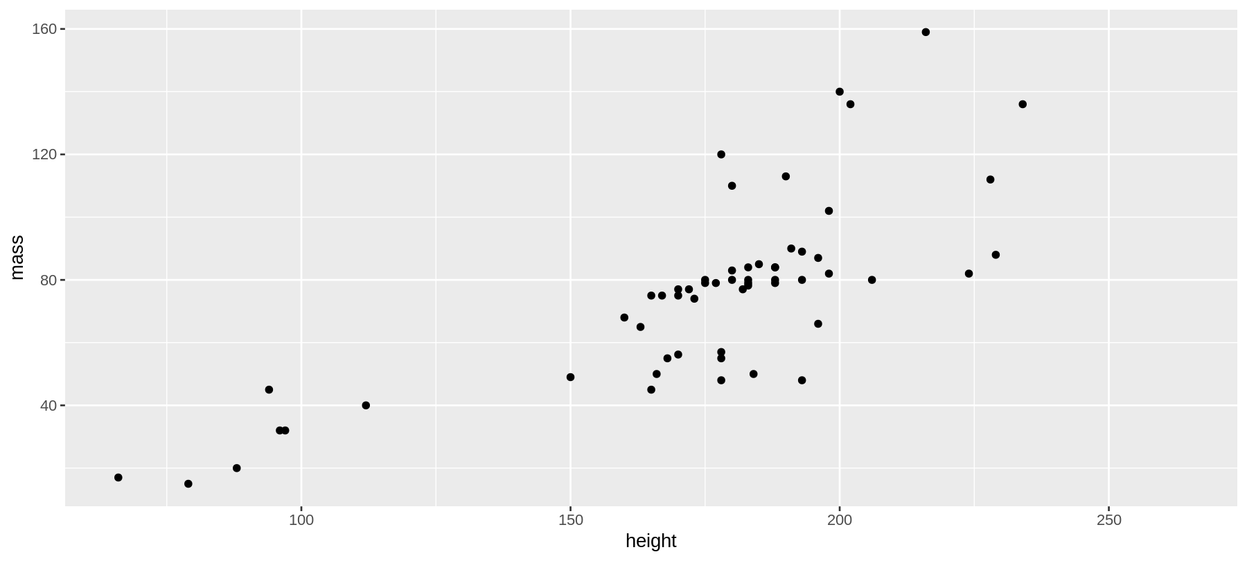
Otsikoiden lisääminen
ggplot(data = sw,
       mapping = aes(x = height,
                     y = mass)) +
  geom_point() +
  labs(title = "Kuvan otsikko", #<<
       x = "pituus", #<<
       y = "paino") #<<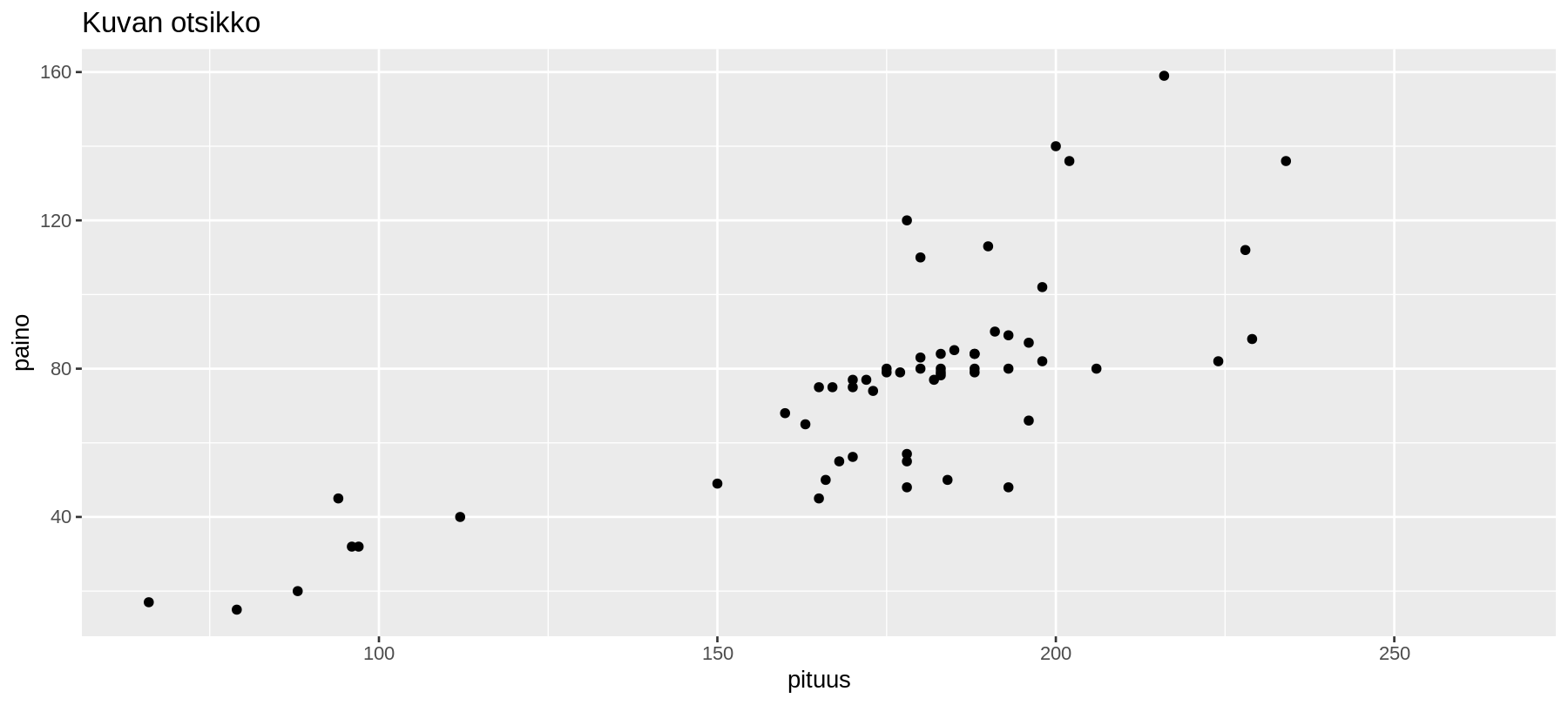
Teeman lisääminen
ggplot(data = sw,
       mapping = aes(x = height,
                     y = mass)) +
  geom_point() +
  labs(title = "Kuvan otsikko",
       x = "pituus",
       y = "paino") +
  theme_minimal() #<<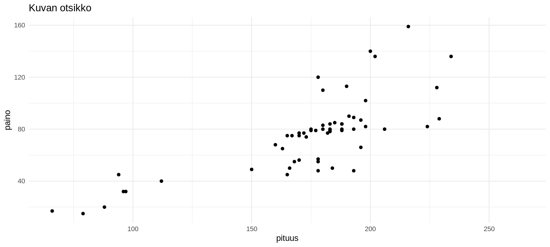
Koordinaatiston vaihtaminen
ggplot(data = sw,
       mapping = aes(x = height,
                     y = mass)) +
  geom_point() +
  labs(title = "Kuvan otsikko",
       x = "pituus",
       y = "paino") +
  theme_minimal() +
  coord_polar() #<<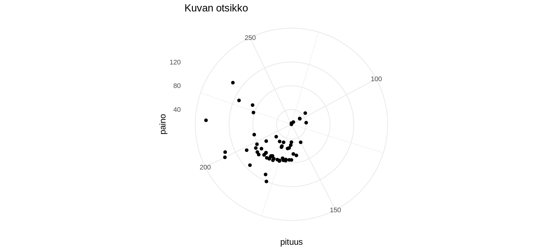
Esimerkkejä erilaisista geometrioista geom_*()
geom_point hajontakuvio
ggplot(data = sw,
       mapping = aes(x = height,
                     y = mass,
                     color = species2)) +
  geom_point() #<<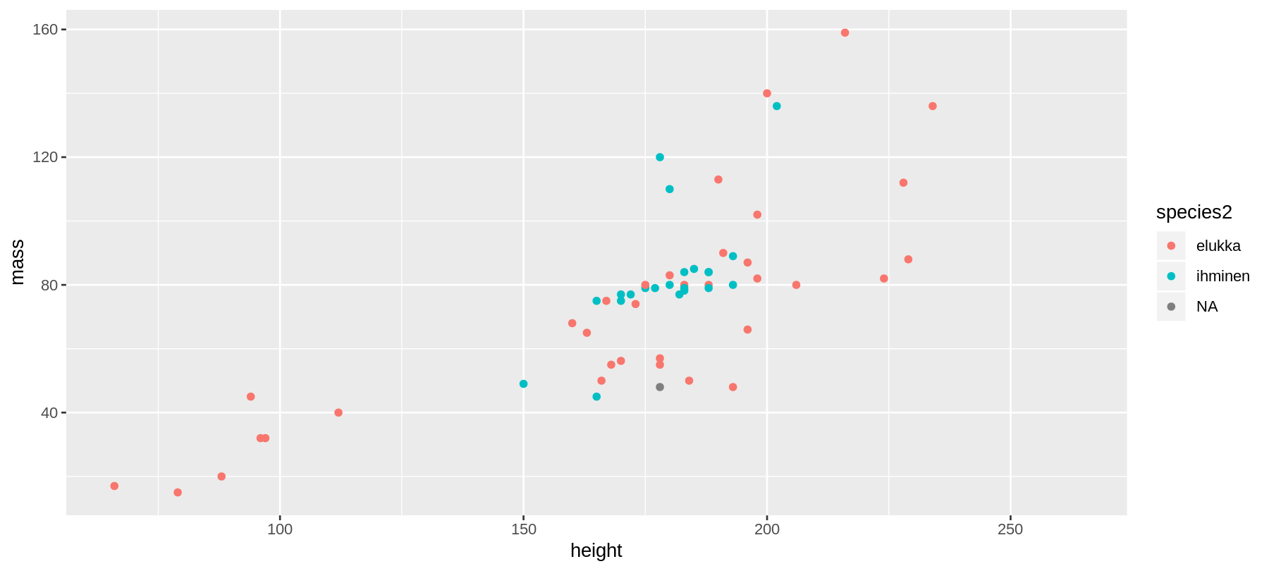
geom_point hajontakuvio ja geom_smooth()
ggplot(data = sw,
       mapping = aes(x = height,
                     y = mass,
                     color =  species2)) +
  geom_point() +
  geom_smooth(method = "lm") #<<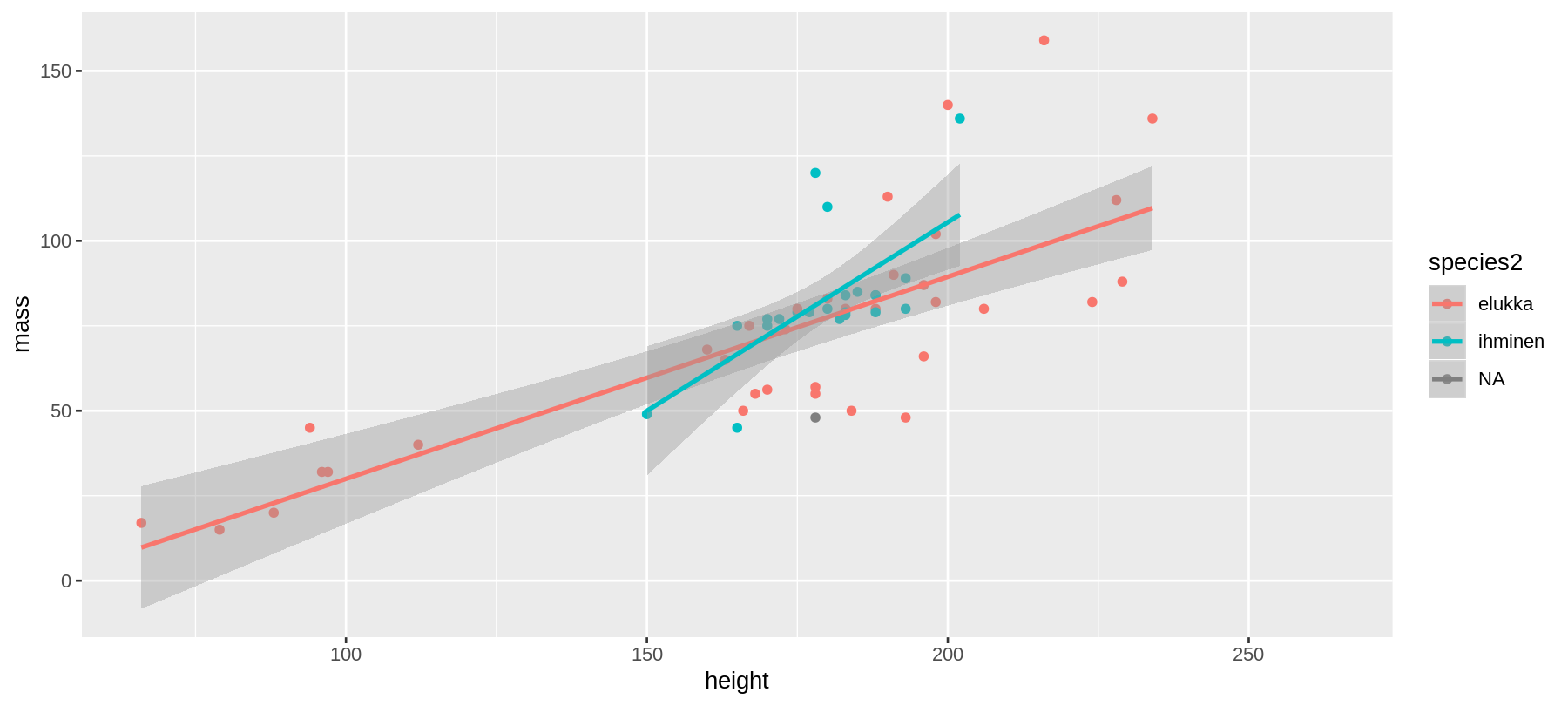
geom_line viivakuvio
ggplot(data = sw %>%
         na.omit(), #<<
       mapping = aes(x = height,
                     y = mass,
                     color =  species2)) + #<<
  geom_line() #<<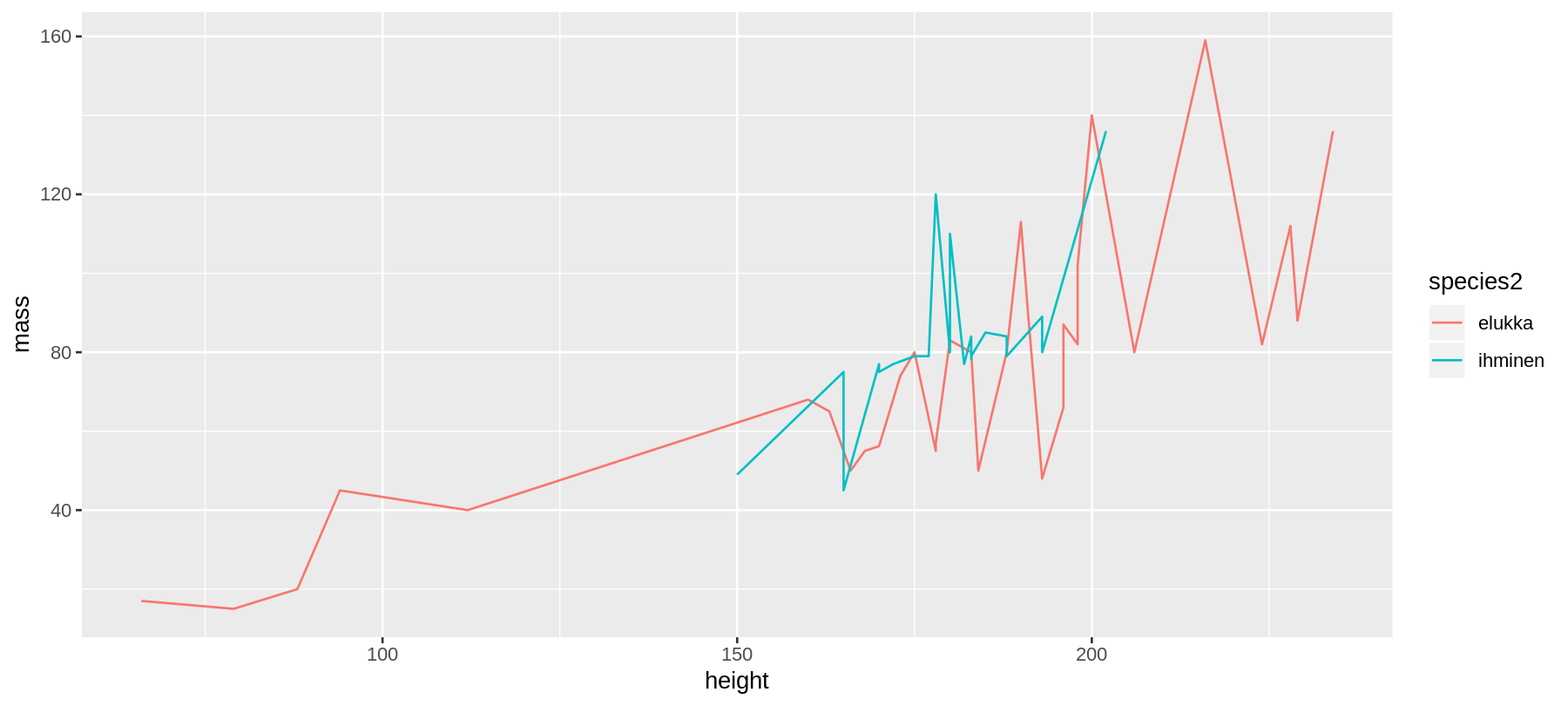
geom_col tolppakuvio
sw %>%
  count(species2) -> d
ggplot(data = d,
       mapping = aes(x = species2,
                     y = n)) +
  geom_col()
geom_histogram()
ggplot(data = sw) +
  geom_histogram(aes(x = height, fill = species2))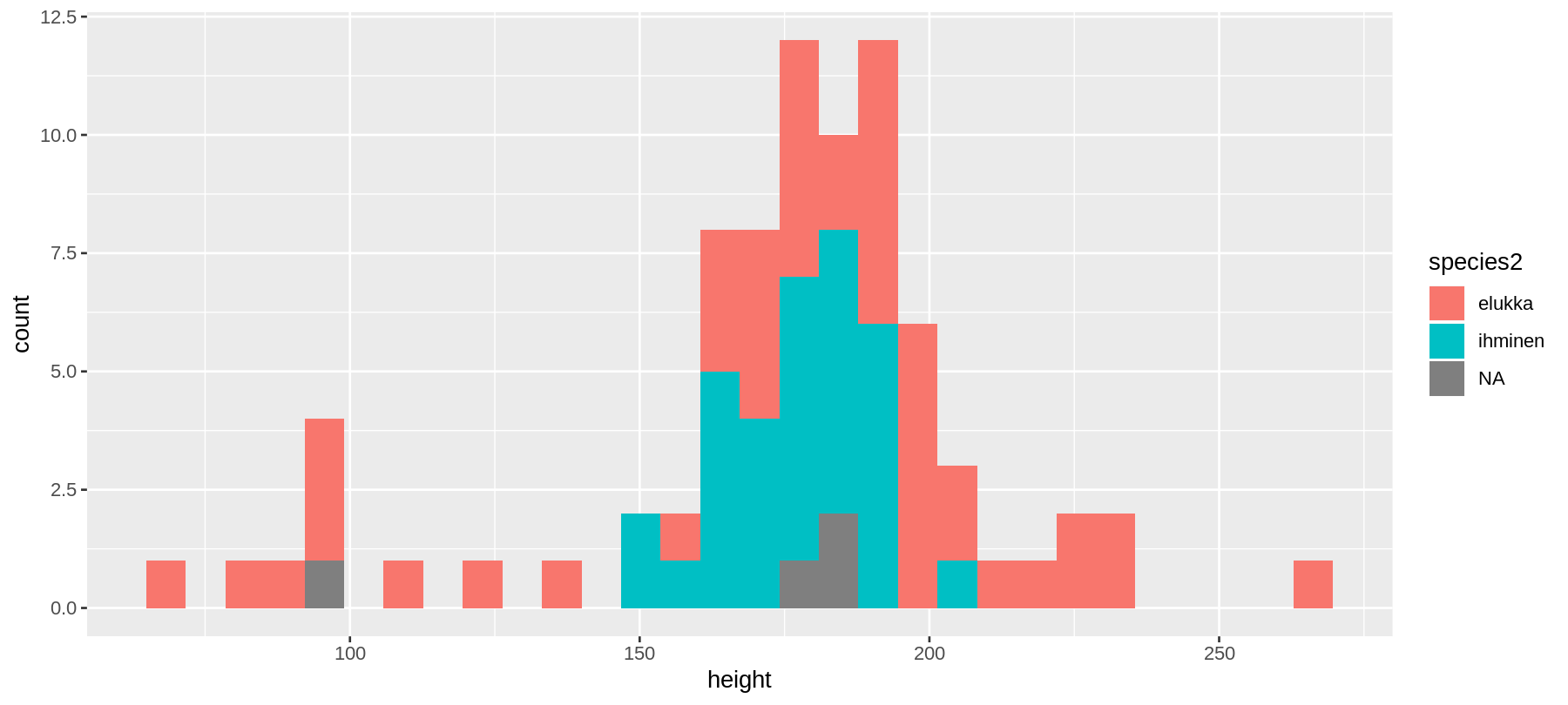
geom_density()
ggplot(data = sw) +
  geom_density(aes(x = height, color = species2))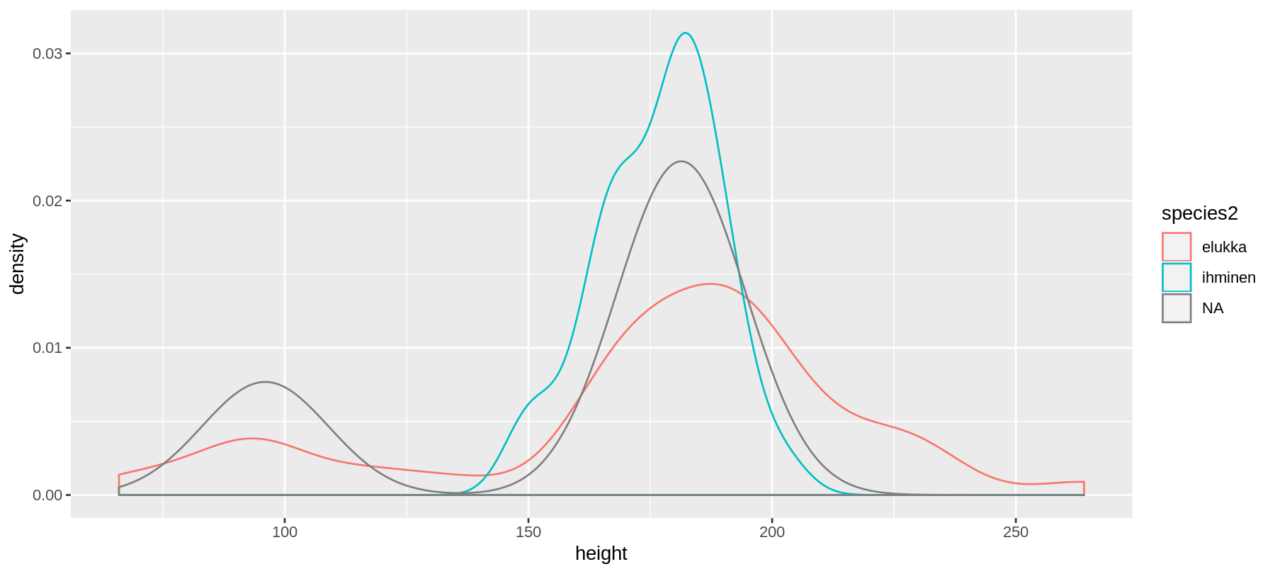
geom_boxplot()
ggplot(data = sw) +
  geom_boxplot(aes(x = species2, y = height))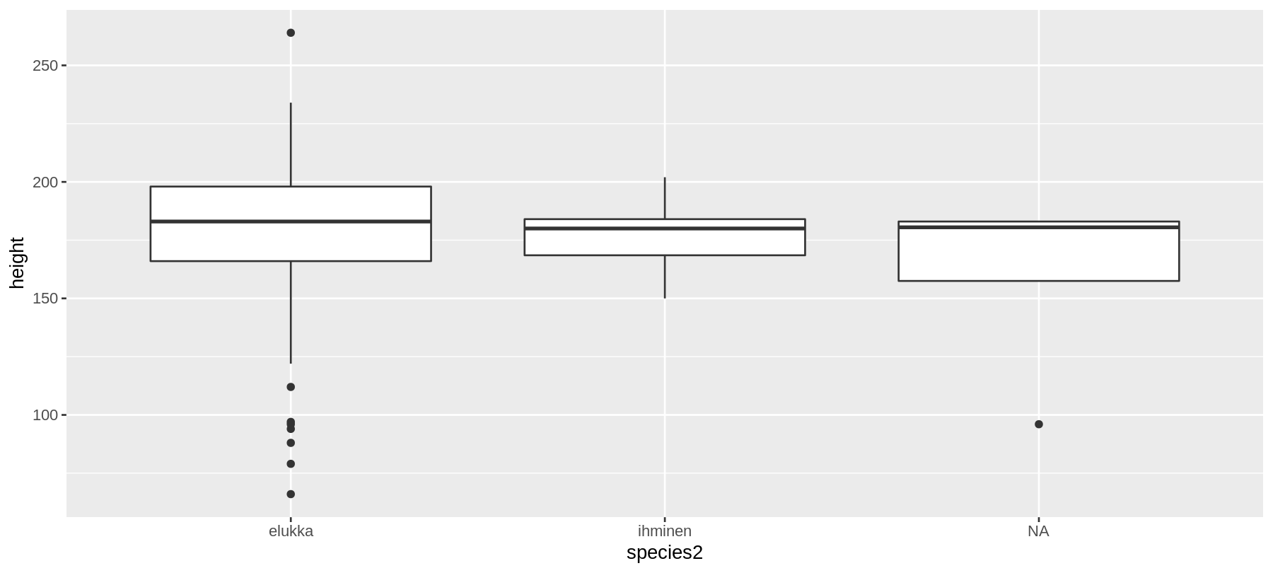
Tilastolliset muunnokset
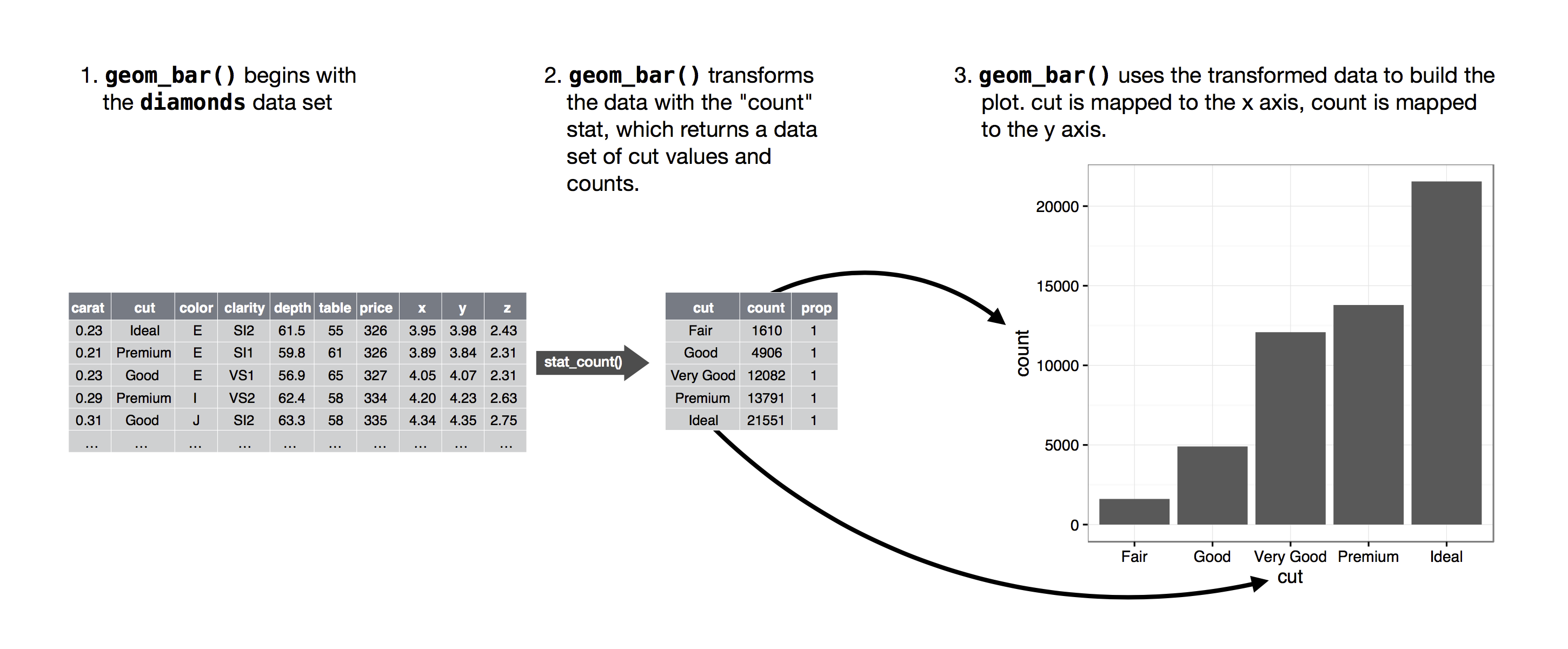
lähde: http://r4ds.had.co.nz/data-visualisation.html#statistical-transformations
data kertauksena
kable(head(sw))| name | height | mass | gender | species2 |
|---|---|---|---|---|
| Luke Skywalker | 172 | 77 | male | ihminen |
| C-3PO | 167 | 75 | NA | elukka |
| R2-D2 | 96 | 32 | NA | elukka |
| Darth Vader | 202 | 136 | male | ihminen |
| Leia Organa | 150 | 49 | female | ihminen |
| Owen Lars | 178 | 120 | male | ihminen |
Tolppakuvio lajimääristä
ggplot(data = sw) +
  geom_bar(mapping = aes(x = species2))
Tolppakuvio lajimääristä niin että datan käsittely erillään
kuvadata <- sw %>% count(species2)
kuvadata
## # A tibble: 3 x 2
## species2 n
## <chr> <int>
## 1 <NA> 5
## 2 elukka 46
## 3 ihminen 35ggplot(data = kuvadata) +
geom_bar(mapping = aes(x = species2, y = n), stat = "identity")
Tolppakuvio lajimääristä geom_col() ilman stat = "identity"
kuvadata <- sw %>% count(species2)
kuvadata
## # A tibble: 3 x 2
## species2 n
## <chr> <int>
## 1 <NA> 5
## 2 elukka 46
## 3 ihminen 35ggplot(data = kuvadata) +
geom_col(mapping = aes(x = species2, y = n))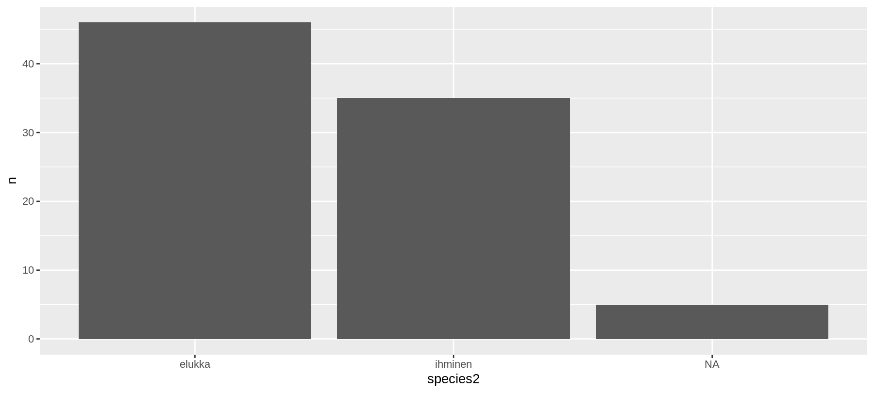
Tolppakuvio lajimäärien suhteellisista osuuksista
ggplot(data = sw) +
  geom_bar(mapping = aes(x = species2, y = ..prop.., group = 1))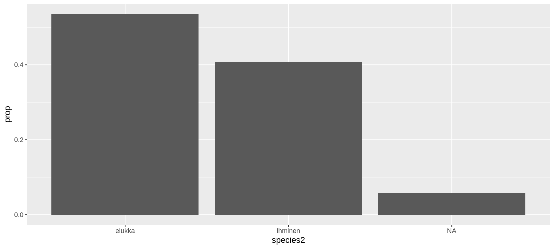
Sama tolppakuvio niin että datan käsittely erillään
kuvadata <- sw %>%
  count(species2) %>%
  mutate(share = n/sum(n))
kuvadata
## # A tibble: 3 x 3
## species2 n share
## <chr> <int> <dbl>
## 1 <NA> 5 0.0581
## 2 elukka 46 0.535
## 3 ihminen 35 0.407ggplot(data = kuvadata) +
geom_col(mapping = aes(x = species2, y = share))
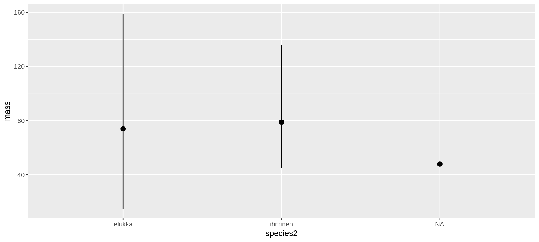
ggplot(data = sw) +
  stat_summary(
    mapping = aes(x = species2, y = mass),
    fun.ymin = min,
    fun.ymax = max,
    fun.y = median
  )
facet_grid()/facet_wrap()-funktiot eli small multiples
facet_wrap()
ggplot(data = sw) +
  geom_point(aes(x = height, y = mass)) +
  facet_wrap(~gender)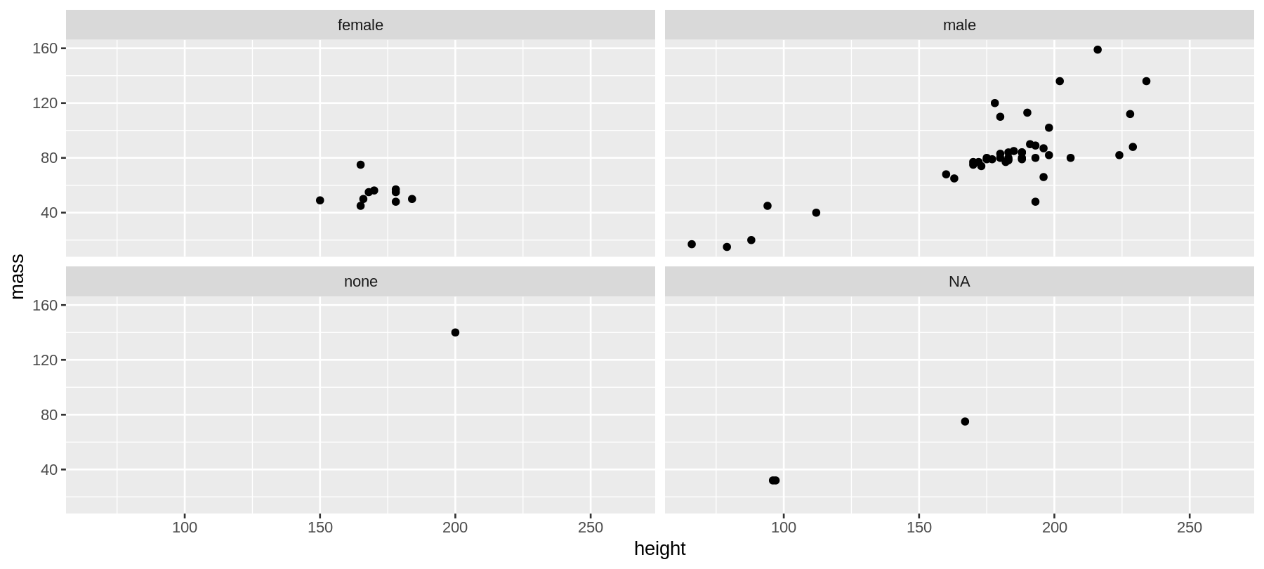
ggplot(data = sw) +
  geom_point(aes(x = height, y = mass)) +
  facet_wrap(~gender+species2) # kaksi muuttujaa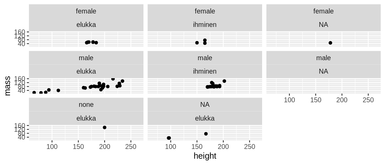
facet_grid()
ggplot(data = sw) +
  geom_point(aes(x = height, y = mass)) +
  facet_grid(species2~gender, scales = "free")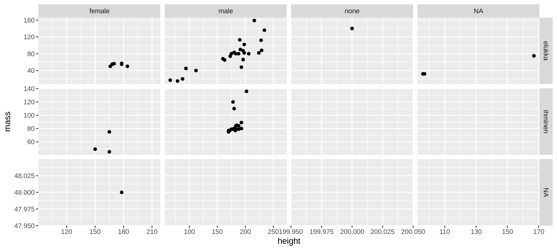
Eri tavat kirjoittaa ggplot2-koodia
# Tapa A
## Koko kuvio yhteen riviin
p <- ggplot() +
  geom_point(data=sw, aes(x=height,y=mass)) +
  geom_smooth()
p


# Tapa B
## Luo kuvio kerros kerrokselta
p <- ggplot()
p <- p + geom_point(data=sw, aes(x=height,y=mass))
p <- p + geom_smooth()
p
Tallenna levylle
ggsave(filename = "tiedosto.png", plot = kuvaobjekti)Lisätietoja
Dokumentaatiota
- Kieran Healy (2019): Data Visualization - A practical introduction
- Winston Chang (2016): R Graphics Cookbook - Practical Recipes for Visualizing Data
- Virallinen dokumentaatio: ggplot2.tidyverse.org
Käyttäjäesimerkkejä
- BBC: How the BBC Visual and Data Journalism team works with graphics in R
- Financial Times (2016): ggplot2 as a Creativity Engine
- Airbnb:n ggplot2-teemapaketti
Ekstra: Twitter-teema
library(ggtech)
ggplot(data = sw %>% na.omit(),
       mapping = aes(x = species2,
                     fill = gender)) +
  geom_bar() +
  labs(title = "Kuvan otsikko",
       subtitle = "Kuvan alaotsikko",
       x = "pituus",
       y = "paino") +
  theme_tech(theme="twitter") +
  scale_fill_tech(theme="twitter") #<<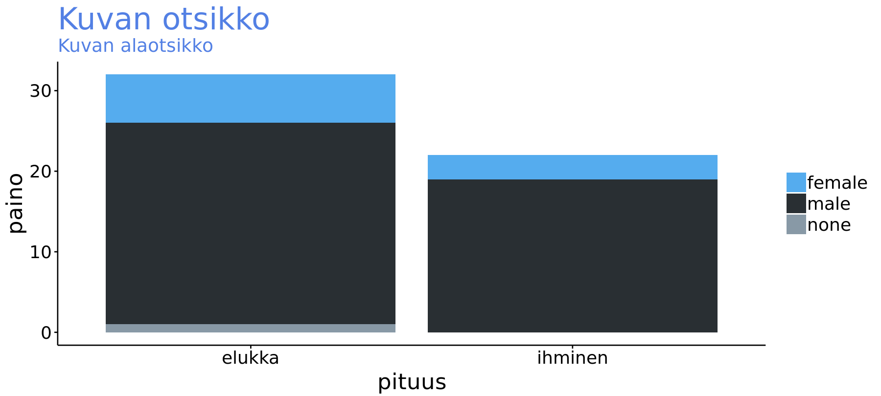
Luento 3: Datan ryhmittely, siivoaminen ja kuvailevat analyysit
Datan siivoaminen ja käsittely dplyr & tidyr -paketeilla
Jos ja kun katsoit jo edellisellä luennolla Garret Grolemundin Data wrangling with R and RStudio niin syvennä tietoutta sitten itse päävelhon Hadley Wickhamin luentojen parissa otsikolla Data manipulation with dplyr osa 1 ja osa 2. Lataa täältä materiaalit luennon harjoitusten tekemiseen!
Jotta voit toistaa videoiden esimerkkejä asenna seuraavat paketit:
install.packages("nycflights13")
devtools::install_github("rstudio/EDAWR")- Kertaa kurssilla läpikäytyjä asioita perehtymällä lukuun 5 Data transformation
- Lataa datan käsittelyn ja siistimisen lunttilappu tästä: Data Transformation Cheat Sheet
Kuvailevat analyysit
Perusteellisempi johdanto ggplot2:n käyttöön on tämä Introduction to ggplot2 in R. Videossa käytetään iris dataa, jonka saat ympäristöösi komennolla data(iris) kun olet ensin ladannut ggplot2-paketin komennolla library(ggplor2). Yrittäkää löytää aika katsoa tämä video!
- Jatka kirjan Data Visualization for Social Science: A practical introduction with R and ggplot2 luvuista 4 Show the right numbers ja 5 Graph tables, add labels, make notes.
- Kertaa kirjasta R for Data Science kappaleesta 3 Data visualisation kohdat 3.1 - 3.4 ja jatka kohtiin 3.5 - 3.10
- Lataa datan visualisoinnin lunttilappu tästä: Data Visualization Cheat Sheet
2017-2019 Markus Kainu.

Tämä teos on lisensoitu Creative Commons Nimeä 4.0 Kansainvälinen -lisenssillä.